Friday Field Photo #182: Stretched-pebble conglomerate

This week’s photo is from Panamint Valley in southeastern California (the valley to the west of Death Valley). This example of a stretched-pebble conglomerate is actually a boulder in a wash and not in place. Therefore, I’m not exactly sure of it’s age, but it’s likely from the Proterzoic Kingston Peak Formation, which crops out in the Panamint range. It’s pretty awesome to think about pebbles in a conglomerate getting deformed and stretched like this.
Happy Friday!
Quick update from EGU 2013
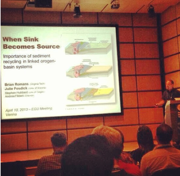 This is my first time attending an EGU (European Geosciences Union) meeting and it’s been great. It’s a rather short trip for the distance traveled — just three nights here in Vienna, Austria — but it has been worth it. The meeting reminds me of the annual AGU meeting held every December in San Francisco, although a bit smaller.
My main motivation for traveling all this way was to give an invited talk in a session convened by Alex Whittaker, Sebastien Castelltort, and Philip Allen called Tectonics, Sedimentation, and Surface Processes yesterday morning. Jon Tennant (@protohedgehog) of the EGU blog Green Tea and Velociraptors took this photo of me (above) beginning my talk.
This talk discussed some new research a close collaborator and good friend of mine is doing comparing crystallization age (U-Pb) and cooling age ([U-Th]/He) of detrital zircons from Magallanes foreland basin (southern Chile/Argentina) sedimentary rocks. Constraining the crystallization age and cooling age of a single zircon grain provides valuable information about the sediment source area, timing of exhumation (when that mineral grain became a sedimentary particle, roughly), and whether or not the grain experienced additional heating through burial.
For this session we used these new data to highlight the recycling of sediments over ~50 million years of fold-thrust belt and foreland basin evolution. The occurrence of recycling of material in such systems has been known for decades, but these newer geo-/thermochronologic techniques can be used to determine the timing/duration of these processes more accurately. For this talk, I discussed these new data within the context of reconstructing ancient sediment-routing (or, source-to-sink) systems. For example, how might recycling of older foreland basin deposits influence our ability to use general grain-size trends to better understand system morphology (e.g., Whittaker et al., 2011)? In the spirit of sharing new ideas and preliminary results I posed more questions than answers in the talk — with the hopes of initiating discussion. I got some great feedback from people throughout the day and ended up having numerous conversations with others doing similar work. This is the whole point of conferences and makes the trip worth it.
My other motivation for attending EGU was to interact with researchers whose work I’ve been following but had not actually met in person yet. It’s great to put faces to names and to get to know people beyond their published papers.
Short Video About IODP Expedition 342 Sampling Party
Last month I traveled to Bremen, Germany along with the rest of the IODP Expedition 342 scientists to help sample the sediment cores we acquired from the bottom of the North Atlantic Ocean last summer. As I mentioned in a post a few weeks ago, the sampling of these archives is a key step for the expedition goals.
The video above (~8 minutes long) does a great job explaining this stage of the science. If the embedded video is not showing up go to this page: http://www.youtube.com/watch?v=J0r2u5xdS7E&feature=youtu.be
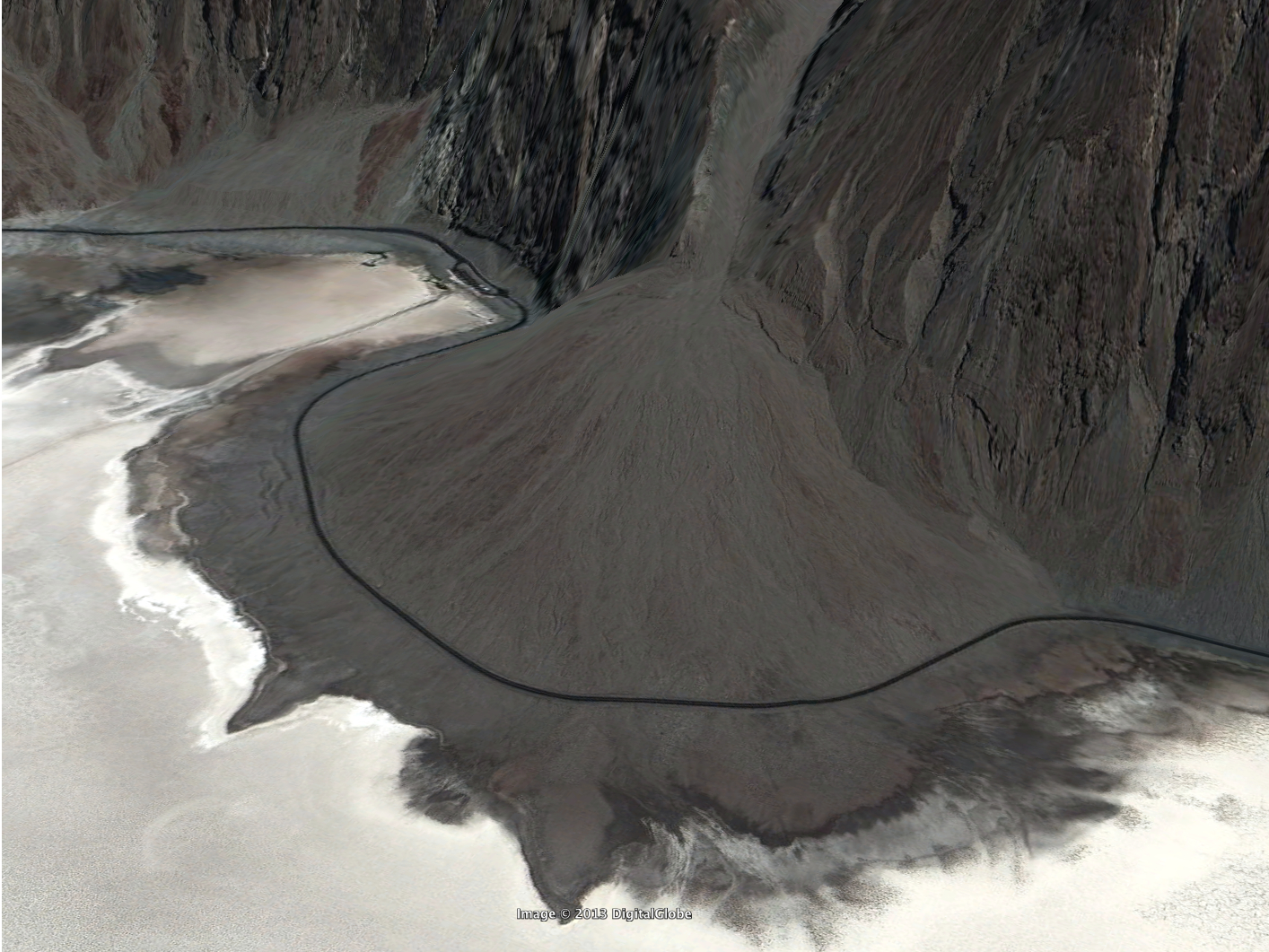
Friday Field Photo #181: Fault Scarps on Badwater Fan

This week’s photo features a rather famous alluvial fan, the Badwater Fan just south of the tourist stop in the lowest spot in the continental United States (at -282 ft) in Death Valley National Park. The east side of Death Valley has numerous small and steep (for depositional systems) alluvial fans. These piles of sediment are aggrading as fast as they can to keep up with the basin dropping out from under them. Further evidence of the movement along the boundary fault (between the uplifting range and the downdropping basin) are the fault scarps in the photo above. Good stuff.
Here are a couple GoogleEarth snapshots of this fan.

Happy Friday!
More photos from a trip to Death and Panamint Valleys here.
IODP Expedition 342 Sampling Party
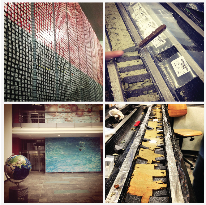
I’m not sure why this event is called a sampling ‘party’, unless you considering extracting various-sized bits of mud from core several hours of day for a week to be a party. More like a sampling binge. That doesn’t mean it wasn’t a great experience, it definitely was. It was fantastic to reconnect with all the great colleagues and friends I made after two months on the JOIDES Resolution last summer. And, of course, a team of >30 scientists working in two shifts at 5-7 stations can get a lot of work done.
The sampling party is a critical component of any Integrated Ocean Drilling Project (IODP) expedition. After all, the whole point of an expedition is to acquire samples of material (sediment and/or rock) from the ocean floor and below. Although a tremendous amount of work is done on the ship as the cores are collected (see the expedition preliminary report here) the expedition itself is really just the beginning.
The overarching goal of Expedition 342 is to examine several of Earth’s climate events/transitions from the Paleogene period (~65 to 23 million years ago) at high resolution. That is, we already know quite a bit about events like the Paleocene-Eocene Thermal Maximum (PETM) and the Eocene-Oligocene transition; however, most records are at temporal resolutions that make it challenging to understand dynamics and effects at shorter timescales. These past events are like ‘experiments’ that the Earth conducted and we need to use them to better understand current, and possibly future, global change. Paleoclimatologists have been able to obtain higher resolution (thousands to tens of thousands of years) with archives from the past two million years (the Quaternary), so another way to put this is: we want to do Quaternary-style paleoclimate analysis on much older records. To make a long story short — this goal requires A LOT of samples. I’m not sure what the latest number is, but it’s something on the order of 50,000 total samples.
Although their is an overarching goal, each scientist has a specific request in terms of what time interval, and what resolution, and how much material they need. As a result, the sampling plan is highly coordinated and the cores are brought out in a systematic fashion to ensure samples are taken as efficiently as possible. (IODP staff are quite good at this.) What’s really great about the sampling party is that the entire science party pitches in. You don’t show up to get just your own samples and then take off. For example, several people on the other shift or working at another station would be taking my samples and I would be taking theirs. And the discussions during sampling were great — a mix of serious science with lots of joking around, which helped maintain some sanity while doing very repetitive tasks.
What’s next? Well, once we all get our samples into our respective labs the analysis will commence. The majority of these samples will be used to generate various isotope data that are useful as climate proxies. Others will be examining the paleobiology/paleoecology of the different types of microfossils and others still will examine ocean chemistry preserved in the sediment. I will be measuring grain size of the terrigenous (land-derived) fraction to better understand the history of the long-lived current that brought sediment to the site. I still have much work to do to get my lab fully operational and the methods perfected, but progress is being made.
Photos: Upper left — stacks of core in the refrigerator; Upper right — in the process of taking 30 cubic centimeter samples; Lower left — lobby of Bremen Core Repository; Lower right — what’s left of one of the cores after sampling. All photos taken by me with my iPhone.
Hanging out with your data
In my never-ending quest to be more productive in my research I notice things about the way I work. I don’t know about others, but I have a difficult time diving back into a project that I haven’t worked on for a few weeks or longer. At least, picking up where I left off with the same momentum. Whether it’s sifting through data, drafting figures, or the actual writing it takes me some time to ‘get into it’. How much time? Depends. In some cases, I can jump back into the very same task and state of mind within ~10-15 minutes. In other cases, I’ll spend an hour (sometimes much longer) flailing about and making little tangible progress.
In the cases where it takes longer to find that groove, I find myself hanging out, for lack of a better phrase, with my data. Not necessarily analyzing it or doing anything useful with it. Just hanging out and being near it. For example, I’ll print out some key outcrop photos, a map, or a plot I made weeks prior and have it near me while I work on unrelated tasks. The questions, ideas, and speculations related to that problem then begin to re-occupy my thoughts. Sooner or later, I’m in the state where I can devote mental effort and make real progress.
Does anyone else work like this?
Update from the field
All is well here in Patagonia. I can only spend a little over a week down here this season (because of teaching obligations), but my graduate student will be staying for several weeks. We’ve spent a few days getting the big picture, the lay of the land so to speak — we will now spend a few days collecting some data (measured sections capturing cm-scale sedimentology along with detailed stratigraphic correlation at the 10s-100s of meters lateral scale). The weather is pretty typical — very windy, scattered rain showers — however, it’s much warmer than usual, into the low 70s F.
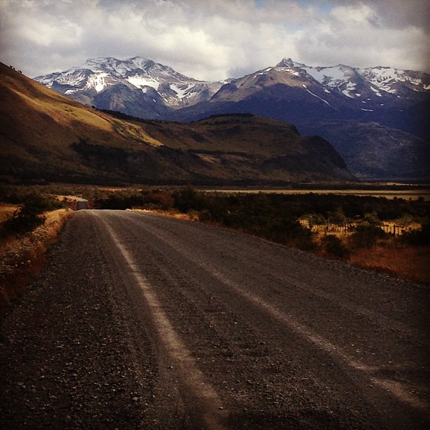
Friday Field Photo #180: Cerro Ventana in Patagonia
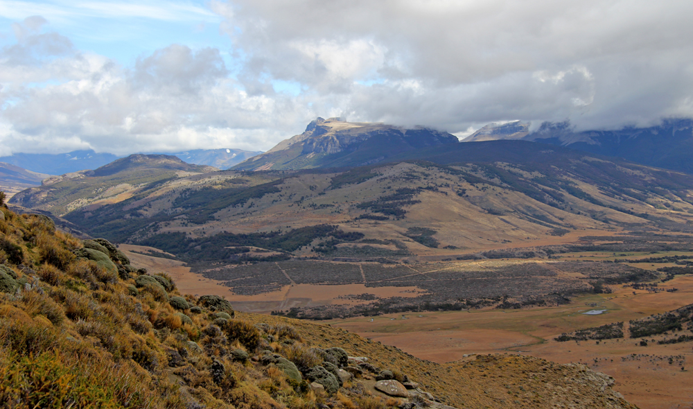
We are getting geared up for another field season in Patagonia — we’ll be looking at these views a week from now! The mountain in the center on the other side of the valley is called Cerro Ventana and is capped by a thick (~300 m) sequence of Upper Cretaceous conglomerate and sandstone of the Cerro Toro Formation. Off in the further distance, and shrouded by clouds, are older rocks (Jurassic to Lower Cretaceous) in the more structurally deformed part of the fold-thrust belt.
Happy Friday!
Can you describe your science using common words?
Every once in a while the internet produces something elegant. Here’s a simple and, in my opinion, brilliant web text editor that forces you to use only the 1,000 most common words in the English language.
Here’s my attempt at describing my research:
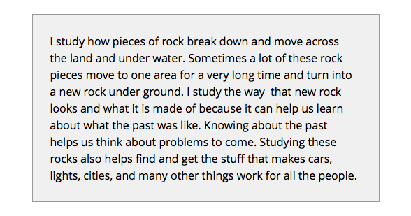 Try it. Whether or not you are satisfied with the result, I think going through this intellectual exercise is worth it. I was forced to pause and think about what word to use several times. I’ve already passed this on to my graduate students and some colleagues. I will definitely use this in the future for teaching as well.
Highly Allochthonous is compiling a list of examples from many geoscientists.
Creating Data Plots with R
First things first, I’m a novice when it comes to coding/programming. So, those of you who are much better at this are free to point and laugh at my lack of skills. I’ve gotten used to revealing my ignorance on a nearly daily basis, which is fine because the more that I do that the more I learn useful stuff.
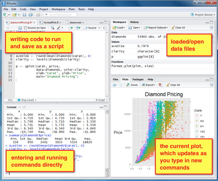
I’ve recently started playing around with the free statistical/graphical programming language and software R. (Here’s some good intro documentation.) For a sampling of what the graphics look like, check out this image gallery. I use R through the separate RStudio interface, which I like quite a bit. This image is from the RStudio website with my own text annotation explaining what the four panels are for.
For this first foray into R I’m interested in creating a simple line plot with custom annotation for some grain-size data I have. Down the road I’d like to learn more about statistical analyses with R, but for now I just want to make some nice-looking graphics for a paper I’m writing.
I’m not sure how many of you who read this blog use R, but I thought it might be fun and mutually helpful to start sharing some ideas and code. Just about everything I’ve learned so far (which is the tip of the tip of the R iceberg) was found by googling various commands. There are numerous sites, forums, and blogs out there with people helping each other out. It’s amazing. However, even with all those resources it’s still sometimes difficult to find exactly what you need. This is especially true for a beginner (i.e., me) who isn’t familiar with all the commands yet.
