Wish list of digital ‘tools’ for stratigraphic analysis
Matt Hall and Evan Bianco of Agile Geoscience recently ran a two-day ‘hackathon’ where participants got together in a room and created some digital tools for working with geophysical data of subsurface geology. It’s a great idea — get some creative and passionate geoscientists and programmers (many participants are both of those) into the same room for a couple of days and build something. And they did.
The success of the Geophysics Hackathon has initiated discussion among the more stratigraphically oriented subsurface interpreters to have a similar event. The when, where, how, and other logistical matters need to be figured out. It takes a critical mass of interested people willing to do the leg work to make stuff like this happen, so we’ll see what happens.
But, for this post, I figured I would brainstorm some digital tools (apps?) that I would love to have for the work I do. Some may be easy to deal with, some may not … it’s a wish list. My focus is on outcrop-derived data because outcrop-based stratigraphy is a focus of my research group. But, these outcrop data are used directly or indirectly to inform how subsurface interpreters make predictions and/or characterize their data.
- Tools for converting outcrop measured sections (and core descriptions) into useable data. To me, this is the primary need. I could envision an entire event focused on this. As outcrop stratigraphers, we typically draft up our 1-D measured sections from scanned images of our field notebooks into a figure. There is value in simply looking at detailed section of sedimentological information in graphic form. This is why we spend time to draft these illustrations. However, we also need to extract quantitative information from these illustrations (an image file of some kind) — information including bed thickness stats, facies proportions, grain-size ‘logs’, package/cycle thickness stats, and more. The key is it has to flexible and able to work with an image file. That is, the data extraction workflow cannot dictate how the original data is collected in the field or how the section is drafted. Sections are drafted in different ways, at different resolutions, and are dependent on the exposure quality, purpose of study, etc. The post-processing must be able to deal with a huge variety.
- Tools for processing outcrop/core data (above) and generating metrics/statistics. Whether integrated into a single tool or as part of a multi-step workflow, we then need some tools that automate the processing of the outcrop/core data to generate metrics we are interested in. For example, if I have 10 sections and I want to calculate the percentages of various facies (e.g., as different colors in image or based on a grain-size log), it would be amazing to have script to automate that.
- A simple and accurate ‘ruler’ app for subsurface visualization software. I find myself constantly wanting to do quick (but not dirty, I want it to be accurate) measurements of dimensions of stratigraphy of interest. Some software packages have built-in rulers to make measurements and some of these are okay, but it’s usually clunky and I end up unsatisfied. I want to know how wide (in meters) and how thick (in TWT milliseconds) something is in seismic-reflection data? And I want it in a matter of seconds. Launch the app, a couple clicks, and I got it. I can move on and don’t have to mess around with any display settings. And if I want to do the same on a different subsurface visualization software, I can use the same app. I have no idea if this is even possible across multiple proprietary software packages, but this is what I want.
Please add comments, write your own post, start a wiki page, etc. to add to this.
Grain Settling Equations and Plots With R
Zoltan Sylvester wrote a nice post a couple weeks ago exploring grain settling equations. He plotted up these equations using some Python code. Here, I simply reproduce what Zoltan did but with R code. So, go read Zoltan’s post first. This was more of an exercise in continuing to learn R rather than an exploration of grain settling physics. And, in this case, doing the ‘translation’ is a nice introduction to how Python works.
My R code works (yay), but seems bulky and cumbersome (boo). I’m sure there are ways to streamline it, feel free to comment with suggestions.
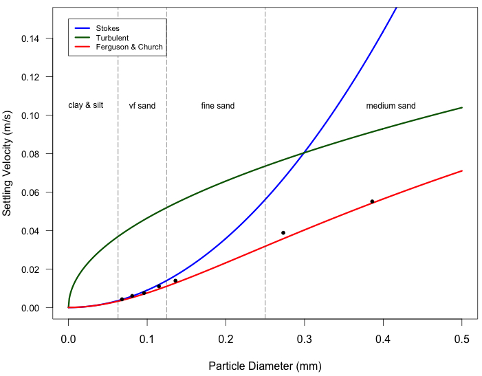
This first box of code defines constants, the three equations to be plotted, and then applies those equations to a range of particle sizes (diameters from 0 to 0.5 mm).
# Some constants for the equations
rop = 2650.0 # density of particle in kg/m^3
rof = 1000.0 # density of water in kg/m^3
visc = 1.002*1E-3 # dynamic viscosity in Pa*s at 20C
C1 = 18 # constant in Ferguson-Church equation
C2 = 1 # constant in Ferguson-Church equation

# Stokes
v_stokes = function(d){
  R = (rop-rof)/rof # submerged specific gravity
  w = R*9.81*(d^2)/(C1*(visc/rof))
  return(w)
}
# Turbulent
v_turb = function(d){
  R = (rop-rof)/rof
  w = ((4*R*9.81*d)/(3*C2))^0.5
  return(w)
}
# Ferguson-Church equation
v_ferg = function(d){
  R = (rop-rof)/rof
  w = ((R*9.81*(d^2))/(C1*(visc/rof)+
      (0.75*C2*R*9.81*(d^3))^0.5))
  return(w)
}

# Define a range (sequence) of particle diameters
d = seq(0,0.0005,0.000001)

# Invoke the function for that range of particle diameters
ws = v_stokes(d)
wt = v_turb(d)
wf = v_ferg(d)
This next box then creates the plot shown below the code.
# Plot diameter (in mm) vs. settling velocity for diameters 0-0.5 mm
plot(d*1000, ws, ylim=c(0,0.15), type="l", lwd=3, col="blue",
     xlab="Particle Diameter (mm)",
     ylab="Settling Velocity (m/s)", yaxt="n")
lines(d*1000, wt, col="darkgreen", lwd=3)
lines(d*1000, wf, col="red", lwd=3)
# Axes labels, ticks, annotation, legend
axis(2, at=seq(0,0.14,0.02), cex.axis=0.85, las=1)
abline(v=c(0.063,0.125,0.250), col="gray40", lwd=0.9, lty=5)
text(0.022,0.105, "clay & silt", cex=0.75)
text(0.094,0.105, "vf sand", cex=0.75)
text(0.190,0.105, "fine sand", cex=0.75)
text(0.410,0.105, "medium sand", cex=0.75)
legend(0,0.15,legend=c("Stokes","Turbulent","Ferguson & Church"),
       cex=0.7, lty=c(1,1,1), lwd=c(3,3,3), col=c("blue","darkgreen","red"))
# Plot points from Table 2 of Ferguson & Church
D = c(0.068,0.081,0.096,0.115,0.136,0.273,0.386,0.550,0.770,1.090,2.180,4.360)
W = c(0.00425,0.0060,0.0075,0.0110,0.0139,0.0388,
     0.0551,0.0729,0.0930,0.141,0.209,0.307)
points(D,W, pch=20)
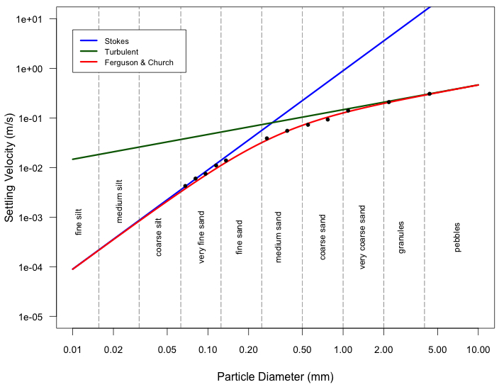
The next part is the same equations but for an expanded range of particle diameters (up to pebbles) and plotted in log-log space.
# Define a range (sequence) of particle diameters
d = seq(0,0.01,0.00001)

# Invoke the function for that range of particle diameters
ws = v_stokes(d)
wt = v_turb(d)
wf = v_ferg(d)

# Plot in log-log space
plot(d*1000, ws, ylim=c(0.00001,10), xlim=c(0.01,10), type="l", log="xy",
     lwd=3, col="blue", xlab="Particle Diameter (mm)",
     ylab="Settling Velocity (m/s)", xaxt="n", yaxt="n")
lines(d*1000, wt, col="darkgreen", lwd=3)
lines(d*1000, wf, col="red", lwd=3)
# Axes labels, ticks, annotation, legend
axis(2, at=c(0.00001,0.0001,0.001,0.01,0.1,1,10), cex.axis=0.85, las=1)
axis(1, at=c(0.01,0.02,0.05,0.1,0.2,0.5,1,2,5,10), cex.axis=0.85, las=1)
abline(v=c(0.0156,0.031,0.063,0.125,0.250,0.5,1,2,4), col="gray40", lwd=0.9, lty=5)
text(0.011,0.0008, "fine silt", cex=0.75, srt=90)
text(0.022,0.0021, "medium silt", cex=0.75, srt=90)
text(0.043,0.0004, "coarse silt", cex=0.75, srt=90)
text(0.09,0.0004, "very fine sand", cex=0.75, srt=90)
text(0.17,0.0004, "fine sand", cex=0.75, srt=90)
text(0.33,0.0004, "medium sand", cex=0.75, srt=90)
text(0.7,0.0004, "coarse sand", cex=0.75, srt=90)
text(1.4,0.0004, "very coarse sand", cex=0.75, srt=90)
text(2.7,0.0004, "granules", cex=0.75, srt=90)
text(7,0.0004, "pebbles", cex=0.75, srt=90)
legend(0.01,6,legend=c("Stokes","Turbulent","Ferguson & Church"),
       cex=0.7, lty=c(1,1,1), lwd=c(3,3,3), col=c("blue","darkgreen","red"))
# Plot points from Table 2 of Ferguson & Church
D = c(0.068,0.081,0.096,0.115,0.136,0.273,0.386,0.550,0.770,1.090,2.180,4.360)
W = c(0.00425,0.0060,0.0075,0.0110,0.0139,0.0388,
      0.0551,0.0729,0.0930,0.141,0.209,0.307)
points(D,W, pch=20)
Comparing Zoltan’s Python code to my R code is a great way to see how each language works.
I’ve been working with and thinking a lot about the silt range of grain sizes lately … look for a post in the future focused on that.
See all my posts about R here.
–
(You probably see an advertisement right below the post. Sorry to clutter up this content with annoying ads, I don’t like it either, but I would otherwise have to pay for hosting. This option is the least intrusive.)
Friday Field Photo #187: Lava Channel on the Big Island

As an Earth scientist who studies surface processes I’m fascinated by channels. Channels are found all over the Earth’s surface, on land and in the deep sea, and we have mapped ancient and active channels on the surface of other planets/moons. As a sedimentary geologist I typically ponder the types of channels that shape landscapes and seascapes, move sediment across the surface, and serve as long-term repositories of deposited sediment.
This week’s photo is indeed a channel but instead of moving sediment it moved molten rock across the surface of the Big Island in Hawaii. It’s now frozen in time, an abandoned channel, perhaps it will be reoccupied by younger lava flows someday. I don’t know the first thing about lava channels, but it seems that it must solidify from the edges inward, resulting in the down ‘stream’ texture (?).
Happy Friday!
–
This photo and more from the Big Island on my Flickr page.
My first post about using R back in January focused on creating custom plots and led to some interaction with other R users in the comment thread and this post from R expert Gavin Simpson in which he kindly offered a solution (and code) to what I was trying to do. I ended up using a slightly modified version of that code to make a bunch of plots for a paper I’m working on. (In fact, I should be working on that paper right now … yep.)
Anyway, for this post I want to briefly summarize another aspect of R (or most programming languages for that matter) that is quite powerful: automating data processing and/or computational tasks that need to be done for multiple files. This funny graphic* below was going around some months ago and very nicely illustrates what I’m talking about.

Just a bit of background before I get on to the R code. I’m starting some research that will take me and my current/future students at least a few years, perhaps more, to accomplish simply because of the huge number of samples. I have a literal boatload of deep-sea sediment samples from IODP Expedition 342 (see this post for context) that will be used to better understand the history of deep ocean circulation in response to past climate change. Specifically, we’ll be measuring the variability in grain size of the terrigenous (land-derived, non-biogenic) sediment through time. To the naked eye, all this sediment is mud. But, subtle differences in the mean size of the silt fraction over time can tell us about the relative intensity of long-lived abyssal currents that transported the sediment. (If you want to know more about this approach, including all the assumptions, limitations, and caveats, this is a nice review.)
Friday Field Photo #186: Coastal California Turbidites

It’s been two years since we moved from California to Virginia, time flies! We really love where we live now, but there are times where I do miss California. I especially miss exploring the outcrops along the coast. Many of these wave-washed bluffs have gorgeous exposures of bed-scale sedimentary geology, a real delight for those who like sedimentary structures.
The above photo shows some Paleocene turbidites along beach cliffs in the town of Gualala, a few hours north of the Bay Area.
Happy Friday!
Friday Field Photo #185: Las rocas del otro lado del río

This photo is from the past field season in Patagonia. We wanted to get to these rocks on the other side of the river. My student eventually got there … by going ~30 km downstream to where there was a proper bridge and then driving on some gnarly roads for a couple hours. If only we had jet packs. Drones are all the rage these days … drones shmones, I want jet packs!
Happy Friday!
Summertime research in the lab

Summer is in full swing and this summer is all about lab work. An undergraduate researcher and I are in the midst of extracting the terrigenous (land-derived) sediment from marine sediment. We are interested in the grain-size and compositional characteristics of the terrigenous component to better understand the history of a long-lived oceanic current that transported the sediment. Isolating the terrigenous material means we have to get rid of the other components, namely the biogenic (marine microfossils made of carbonate and opal) and authigenic (metalliferous oxyhydroxides that formed in place) material. We are using this method with some tweaks from a helpful collaborator.
I have >1,000 samples from IODP Expedition 342 (see this post for more about that expedition) that will eventually be processed in this way. But, because we have not done this before and are still getting the lab fully equipped, we are currently using ‘practice’ sediment (a chunk from one of the core catchers) to fine-tune the methodology. That is, when we make a mistake — which is inevitable when learning something new — we won’t be sacrificing a ‘real’ sample. This training will pay off in a couple weeks as we ramp up and start processing samples in batches.
While we work on that two of my graduate students are busy crushing, grinding, sawing, drilling, etc. rock samples for their respective Ph.D. projects. We’ve got mineral separation underway for bedrock thermochronology, sample preparation for stable isotope measurement of carbonate rocks, and thin sections being made.
Summertime!
Friday Field Photo #184: Death Valley Dunes

Here’s a shot of the sand dunes not far from Stovepipe Wells in Death Valley National Park from this past March. Check out this Flickr set for a whole bunch more. Happy Friday!

This week’s photo is from the deck of the JOIDES Resolution drill ship last summer. Before IODP Expedition 342 I had spent only a few days at sea, and even then it wasn’t more than ~20-30 km from land. Being out in the open ocean — several hundred km from land — was an experience I didn’t think about or appreciate before I did it.
I never grew tired of watching the sea during that two months. The interaction of swells of different sizes and forms moving in different directions resulted in unique displays of nature. And it’s quite different than watching the sea near the coast. Watching the water pile up into ‘mountains’ and ‘ridges’, creating a constantly changing topography, was actually quite therapeutic during an incredibly busy expedition.
Happy Friday!
See this photo and many more from IODP Expedition 342 on my Flickr page.
Amazing view of the Mississippi River delta

Mississippi River delta from the International Space Station (photo by @Cmdr_Hadfield)
I just had to share this image that Commander Chris Hadfield, an astronaut currently on the International Space Station, posted yesterday. I really like this perspective of the Mississippi River delta. It’s nice to get a view that isn’t a standard map (north to the top and looking straight down). This slightly oblique view emphasizes how ‘delicate’ the bird’s foot part of the delta is, that the boundary between what is land and what is not is a bit blurred.
I’ll also use this post as a plug for Commander Hadfield’s Twitter feed. It’s really quite simple — he takes photos of the Earth out the window of the space station and shares them. There isn’t a link to some busy web page or other social media noise, just a beautiful photo of our planet. And he does several each day. Simple and awesome.
