Grain Settling Equations and Plots With R

Zoltan Sylvester wrote a nice post a couple weeks ago exploring grain settling equations. He plotted up these equations using some Python code. Here, I simply reproduce what Zoltan did but with R code. So, go read Zoltan’s post first. This was more of an exercise in continuing to learn R rather than an exploration of grain settling physics. And, in this case, doing the ‘translation’ is a nice introduction to how Python works.

My R code works (yay), but seems bulky and cumbersome (boo). I’m sure there are ways to streamline it, feel free to comment with suggestions.

This first box of code defines constants, the three equations to be plotted, and then applies those equations to a range of particle sizes (diameters from 0 to 0.5 mm).

# Some constants for the equations
rop = 2650.0 # density of particle in kg/m^3
rof = 1000.0 # density of water in kg/m^3
visc = 1.002*1E-3 # dynamic viscosity in Pa*s at 20C
C1 = 18 # constant in Ferguson-Church equation
C2 = 1 # constant in Ferguson-Church equation

# Stokes
v_stokes = function(d){
  R = (rop-rof)/rof # submerged specific gravity
  w = R*9.81*(d^2)/(C1*(visc/rof))
  return(w)
}
# Turbulent
v_turb = function(d){
  R = (rop-rof)/rof 
  w = ((4*R*9.81*d)/(3*C2))^0.5
  return(w)
}
# Ferguson-Church equation
v_ferg = function(d){
  R = (rop-rof)/rof 
  w = ((R*9.81*(d^2))/(C1*(visc/rof)+
      (0.75*C2*R*9.81*(d^3))^0.5))
  return(w)
}

# Define a range (sequence) of particle diameters
d = seq(0,0.0005,0.000001)

# Invoke the function for that range of particle diameters
ws = v_stokes(d)
wt = v_turb(d)
wf = v_ferg(d)

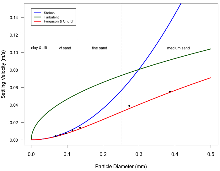
This next box then creates the plot shown below the code.

# Plot diameter (in mm) vs. settling velocity for diameters 0-0.5 mm
plot(d*1000, ws, ylim=c(0,0.15), type="l", lwd=3, col="blue", 
     xlab="Particle Diameter (mm)", 
     ylab="Settling Velocity (m/s)", yaxt="n")
lines(d*1000, wt, col="darkgreen", lwd=3)
lines(d*1000, wf, col="red", lwd=3)
# Axes labels, ticks, annotation, legend
axis(2, at=seq(0,0.14,0.02), cex.axis=0.85, las=1)
abline(v=c(0.063,0.125,0.250), col="gray40", lwd=0.9, lty=5)
text(0.022,0.105, "clay & silt", cex=0.75)
text(0.094,0.105, "vf sand", cex=0.75)
text(0.190,0.105, "fine sand", cex=0.75)
text(0.410,0.105, "medium sand", cex=0.75)
legend(0,0.15,legend=c("Stokes","Turbulent","Ferguson & Church"),
       cex=0.7, lty=c(1,1,1), lwd=c(3,3,3), col=c("blue","darkgreen","red"))
# Plot points from Table 2 of Ferguson & Church
D = c(0.068,0.081,0.096,0.115,0.136,0.273,0.386,0.550,0.770,1.090,2.180,4.360)
W = c(0.00425,0.0060,0.0075,0.0110,0.0139,0.0388,
     0.0551,0.0729,0.0930,0.141,0.209,0.307)
points(D,W, pch=20)

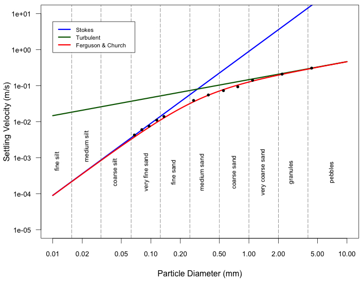
The next part is the same equations but for an expanded range of particle diameters (up to pebbles) and plotted in log-log space.

# Define a range (sequence) of particle diameters
d = seq(0,0.01,0.00001)

# Invoke the function for that range of particle diameters
ws = v_stokes(d)
wt = v_turb(d)
wf = v_ferg(d)

# Plot in log-log space
plot(d*1000, ws, ylim=c(0.00001,10), xlim=c(0.01,10), type="l", log="xy", 
     lwd=3, col="blue", xlab="Particle Diameter (mm)", 
     ylab="Settling Velocity (m/s)", xaxt="n", yaxt="n")
lines(d*1000, wt, col="darkgreen", lwd=3)
lines(d*1000, wf, col="red", lwd=3)
# Axes labels, ticks, annotation, legend
axis(2, at=c(0.00001,0.0001,0.001,0.01,0.1,1,10), cex.axis=0.85, las=1)
axis(1, at=c(0.01,0.02,0.05,0.1,0.2,0.5,1,2,5,10), cex.axis=0.85, las=1)
abline(v=c(0.0156,0.031,0.063,0.125,0.250,0.5,1,2,4), col="gray40", lwd=0.9, lty=5)
text(0.011,0.0008, "fine silt", cex=0.75, srt=90)
text(0.022,0.0021, "medium silt", cex=0.75, srt=90)
text(0.043,0.0004, "coarse silt", cex=0.75, srt=90)
text(0.09,0.0004, "very fine sand", cex=0.75, srt=90)
text(0.17,0.0004, "fine sand", cex=0.75, srt=90)
text(0.33,0.0004, "medium sand", cex=0.75, srt=90)
text(0.7,0.0004, "coarse sand", cex=0.75, srt=90)
text(1.4,0.0004, "very coarse sand", cex=0.75, srt=90)
text(2.7,0.0004, "granules", cex=0.75, srt=90)
text(7,0.0004, "pebbles", cex=0.75, srt=90)
legend(0.01,6,legend=c("Stokes","Turbulent","Ferguson & Church"),
       cex=0.7, lty=c(1,1,1), lwd=c(3,3,3), col=c("blue","darkgreen","red"))
# Plot points from Table 2 of Ferguson & Church
D = c(0.068,0.081,0.096,0.115,0.136,0.273,0.386,0.550,0.770,1.090,2.180,4.360)
W = c(0.00425,0.0060,0.0075,0.0110,0.0139,0.0388,
      0.0551,0.0729,0.0930,0.141,0.209,0.307)
points(D,W, pch=20)

Comparing Zoltan’s Python code to my R code is a great way to see how each language works.

I’ve been working with and thinking a lot about the silt range of grain sizes lately … look for a post in the future focused on that.

See all my posts about R here.

–

(You probably see an advertisement right below the post. Sorry to clutter up this content with annoying ads, I don’t like it either, but I would otherwise have to pay for hosting. This option is the least intrusive.)